Game Theory Examples (ii) - Mixed Strategy Equilibria

Sometimes it is not possible to find a Nash equilibrium using pure strategies, e.g. using iterated removal of dominated strategies. But, in these cases there will be an equilibrium where one or more of the players is mixing their strategies (for finite games).

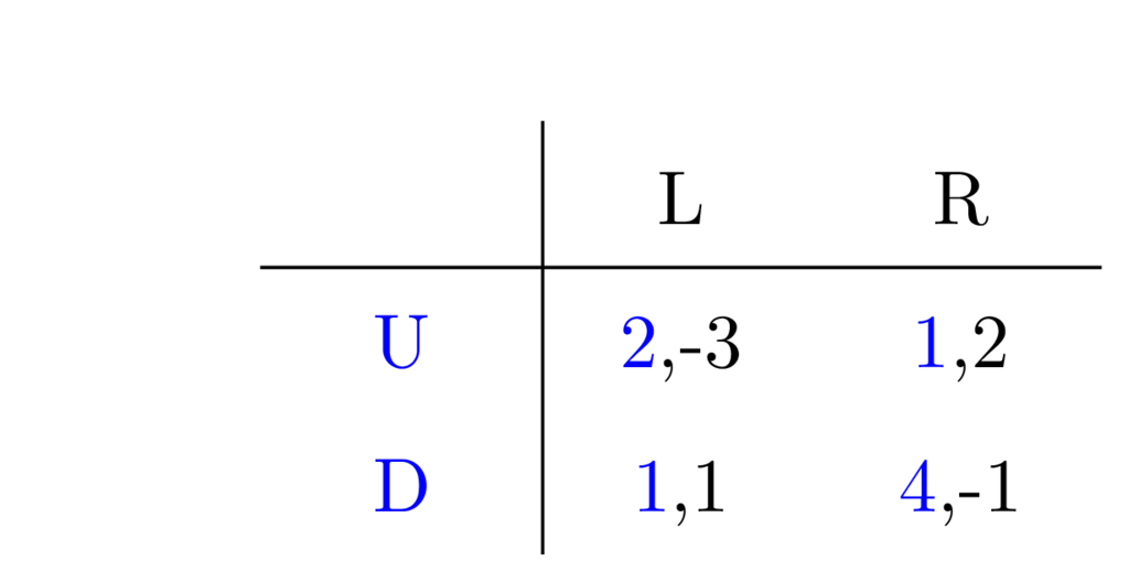
To see what I mean, consider the following game where the row player can choose between the strategies U and D, while the column player can choose between L and R:

There are no dominating strategies among U and D, neither between L and R. In fact, for any cell in the matrix there is one player who will want to move away from it. (Say the strategy combination U-R is picked first. Well, now the column player is satisfied, but the row player thinks they could do better, changing to D, but then the column player will want to change to L, so then the row player changes to U, and …)

But what if strategies could be mixed in the sense that players pick one at random according to some distribution? Then, if the same game is played over and over the players would want to do well on average, and tune the probability by which they choose between strategies accordingly.

Could the expected utility be such that there's a Nash equilibrium (that is a state where none players would not want to pick another of their strategies)?

The strategies U,D, and L,R are called pure strategies while a combination of them is called mixed. A mixed strategy is essentially a probability distribution over each player's strategies.

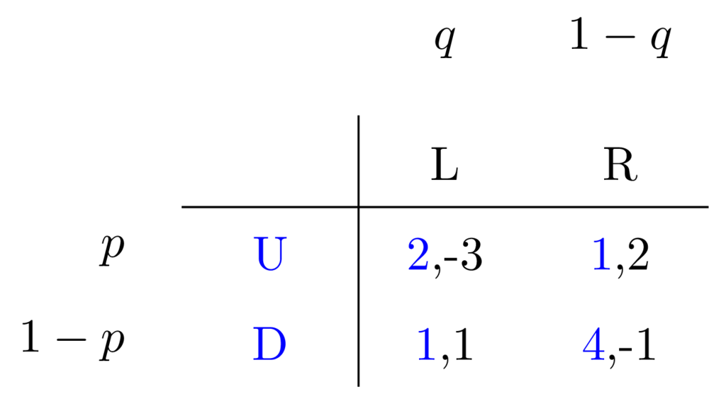
Let's assume that the row player chooses U with probability \(p\), then they must pick the other, D, with probability \(1-p\).

In the same way, assume that the column player picks L with probability \(q\) and R with probability \(1-q\).

Like this:

Our task then is to set up some kind of equation system and solve for \(q\) and \(p\).

The key observation is that for a player to be indifferent to the available strategies, the expected utility those strategies must be equal. Meaning that the row player should determine \(p\) such that their opponent (the column player) expects the same reward from both their available strategies (L and R).

If this isn't the case, then there is always a 'better' choice for the opponent. So, to determine the probability distribution for one player we look at which point the opposing player is indifferent.

In this spirit, let's start by determining the probabilities \(q\) and \(1-q\) for the column player strategies. The above means that for the row player the following must hold \[E\left[U\right] = E\left[D\right].\]

So, what is \(E\left[U\right]\)? Well, with probability \(q\) the column player chooses L, in which case the utility for the row player will be \(2\), and with probability \(1-q\) the column player chooses R, in which case the utility for the row player will be \(1\).

So, if a game is played over and over the row player can expect the following reward on average from strategy U.

\[ E\left[U\right] = 2\times q + 1\times\left(1 - q\right) = q + 1. \]

Using the same reasoning we can see that the row player's expected utility for strategy D is:

\[ E\left[D\right] = 1\times q + 4\times\left(1 - q\right) = 4 - 3q. \]

Now, because the row player must be indifferent we know that \[ q + 1 = 4 - 3q, \] and solving it gives \(q = \frac{3}{4}\).

And here is our answer then. The probability for strategy L is \(q = \frac{3}{4}\), while the probability for strategy R is \(1-q = 1 - \frac{3}{4} = \frac{1}{4}\).

For completeness we then do the same for the row player; calculating \(p\), and \(1-p\). Now we need to see what the expected reward is for the column player.

\[ E\left[L\right] = -3\times p + 1\times\left(1 - p\right) = 1 - 4p, \] \[ E\left[R\right] = 2\times p + (-1)\times\left(1 - p\right) = 3p -1. \]

Then requiring the column player to be indifferent \[E\left[L\right] = E\left[R\right],\] \[1 - 4p = 3p -1,\] from which we have \(p = \frac{2}{7}\).

So, the row player picks strategy U with probability \(p=\frac{2}{7}\), and strategy D with probability \(1-p = \frac{5}{7}\).

That's it. Again, note that the probability for a strategy is computed from the observation that the opposing player must be indifferent.

The basis for this document is a game theory exercise session I taught for an AI course. The notes are quite verbose to start with, because I'm trying to explain every step extensively. Moreover some terms are not directly defined even though I try to explain things on a quite basic level. It was assumed that the students had attended an introductory lecture. So the game is on normal form, 'equilibrium' means Nash equilibrium, and so on. Also please note that in the text I use the terms reward, payoff, and utility interchangeably.

Basically, this is an in-depth example, not a formal introduction.