Braess's 'paradox' and a bit of game theory

Imagine a large number of cars - \(N\) - going at rush-hour every day from some location \(S\) to \(G\). Assume that these are driven by the usual self-interested and perfectly rational beings of Nash-equilibrium game theory we have seen before. (Also let the cars be either full or that there is no car pooling, if you are nit-picky about details.)

So, this is an \(N\) player game. Each driver has a choice of two routes: they can either choose to take the road from \(S\) to point \(a\), and then to \(G\), or they can go from \(S\) to point \(b\) to \(G\). So, there are two strategies: \(SaG\) and \(SbG\). Moreover, for some roads there is congestion so that the cost of commuting (in for example time) is dependent on how many cars are using the road, while for others the cost is constant no matter how many cars are using that particular stretch.

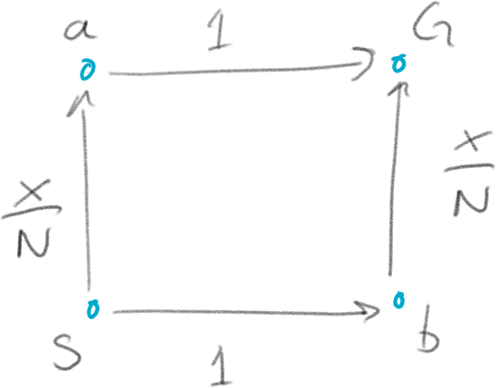
Denote the costs associated with some road segment \(uv\) as \(t_{uv}\), and for the segments listed above associate the costs as in Figure 1 below. Namely

\begin{align*} &t_{Sa}(x) = \frac{x}{N}\\ &t_{aG} = 1\\ &t_{Sb} = 1\\ &t_{bG}(x) = \frac{x}{N}, \end{align*}

where \(x \in [0,N]\) is the number of cars on that road.

In this case each driver wants to minimize their cost (keep this in mind, as often games are thought of as maximizing reward).

Now, the value (= total cost) for strategy \(SaG\) is \(v(SaG) = t_{Sa}(x) + t_{aG} = \frac{x}{N} + 1\), and similarly \(v(SbG) = t_{Sb} + t_{bG}(x) = 1 + \frac{x}{N}\).

As you probably can guess from the symmetry of the game and the two value functions, each of the \(N\) players will minimize their cost by picking a route randomly and with equal probability. This is because when, \(x_a = \frac{N}{2}\) cars go over \(a\) and \(x_b = \frac{N}{2}\) over \(b\), then \[\left. v(SaG) \right|_{x = x_a} = \left. v(SbG) \right|_{x = x_b} = 1 + \frac{N}{2N} = 1.5.\]

If more than \(\frac{N}{2}\) cars take either \(Sa\) or \(bG\) then it is beneficial to change strategy because there will be less cost in going on the opposite. So, the best thing to do is to randomize over the two strategies.

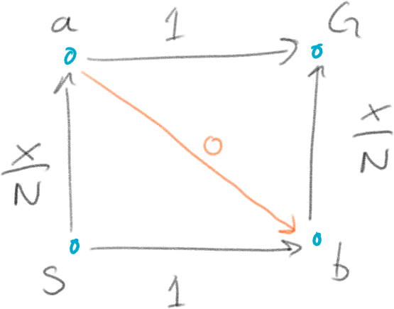
All good this far. But now the traffic authority builds a new super-highway-tunnel from location \(a\) to \(b\). It is really efficient and adds no extra cost to the drivers \(t_{ab} = 0\), as in Figure 2.

This means that there is a new strategy available in addition to the previous two: \(SabG\). That is, first drive from \(S\) to \(a\) then to \(b\) and from there to \(G\).

The value function for the new strategy is quite straight forward: \(v(SabG) = \frac{x}{N} + 0 + \frac{x}{N} = \frac{2x}{N}\).

And, as you might have expected, the equilibrium shifts now that the game has changed. Assume that we start out as before with \(x_a = \frac{N}{2}\) cars driving route \(Sa\). Well, this means that the remaining \(\frac{N}{2}\) cars go \(Sb\), and thus \(x_b = \frac{N}{2}\). So, the best strategy for the cars over \(a\) is to go to \(b\), because the additional cost of this is merely \(0 + \frac{N}{2N} = \frac{1}{2}\) (and going straight \(aG\) costs 1). But now the players going \(Sb\) wants to change. Their total cost is still \(1.5\), while the other drivers get only a total of \(1\).

So, randomly going either \(Sa\) or \(Sb\) is not a Nash equilibrium any more. More drivers will want to go to \(a\). How many?

All of them.

The new equilibrium is simply that every player chooses strategy \(SabG\). The associated cost then \(v(SabG) = \frac{2N}{N} = 2\). You can check this by verifying that no other route will give a lower cost for an individual driver - it will only lower cost for others. There is thus no incentive to change for a perfectly rational driver.

Note that even the individual cost in this equilibrium is more than before (2 > 1.5). Still, nobody wants to change.

The above is an example of what is called Braess's paradox in the study of road networks and traffic flow. It might seem a bit contrived at first, but examples have been reported in traffic. For instance where closing roads or highway lanes might actually improve traffic flow. In general where more resources does not necessarily lead to better outcomes.

It is not quite a 'paradox'. In game theoretic terms it is an example of when the Nash equilibrium does not agree with other types of equilibria. Clearly everyone could be better off by (for example) agreeing not to use the new road, or say by allowing a central route planner to direct which road to use.

You might even ask if there is a correlated equilibrium - where each driver accepts and respects the outcome of some random process assigning new route, leading to an even lower cost over time.

So, let's associate \(P(SaG) = p_1, P(SbG) = p_2, P(SabG) = p_3\), and \(p_1 + p_2 + p_3 = 1\). Given this distribution, let \(E[X_{Sa}], E[X_{bG}]\) denote the expected number of cars between points \(Sa\), and \(bG\) respectively.

Now we can write the expected commuting cost of a player as \(\bar{v} = p_1 v(SaG) + p_2 v(SbG) + p_3 v(SabG) = p_1 (\frac{E[X_{Sa}]}{N} + 1) + p_2 (1 + \frac{E[X_{bG}] + 1}{N}) + p_3 (\frac{E[X_{Sa}]}{N} + 0 + \frac{E[X_{bG}]}{N}).\)

Noting that \(\frac{E[X_{Sa}]}{N} = p_1 + p_3\), and similarly for route \(bG\), we can write the above as.

\(\bar{v} = p_1 ( p_1 + p_3 + 1) + p_2 (1 + p_2 + p3) + p_3 (p_1+p_3 + p_2+p_3) = (p_3 + p_1)^2 + (p_3 + p_2)^2 + p_1 + p_2.\)

Using, e.g. \(p_3 = 1 - p_2 - p_1\), this can be written as \(\bar{v} = 2 + p_1^2 + p_2^2 - p_1 - p_2\), which has a minimum at \(p_1 = p_2 = 0.5\). Thus, the correlated equilibrium is at \(p_1 = 0.5, p_2 = 0.5, p_3 = 0\).

That is, the best thing to do is to stop using the new road completely and allowing the traffic authority to randomly assign a route, which coincidentally happens to be exactly the same as letting every driver randomize without the \(ab\) connection.

I think Braess's paradox is a pretty neat example of how the existence of choice or resources can result in less efficiency as a whole for systems of 'rational agents'.

It's related to more complex flow problems on graphs/networks, and to other applications than traffic.

That said, I think that this simple example might provide an intuition pump also closer to home, when discussing the future of autonomous vehicles. For it is easy to imagine that many potential instances of this paradox has been dampened by human driver 'irrationality'. Choice of route can be down to scenery, joy of driving, or simply overconfidence in knowing the 'best route', or many other things which makes perfect sense when it isn't thought too much about. But then, if everyone buys a car, wouldn't they want the 'best' car, taking the 'best route', just as all the other cars (and already seen with GPS route planners in many places).

But more on that, perhaps, some other time.